Measuring Fitness: Finite Resource Allocation

”To become a science DQ must have a foundation built on measurement.” (Karr, Sanil, and Banks, 2005)

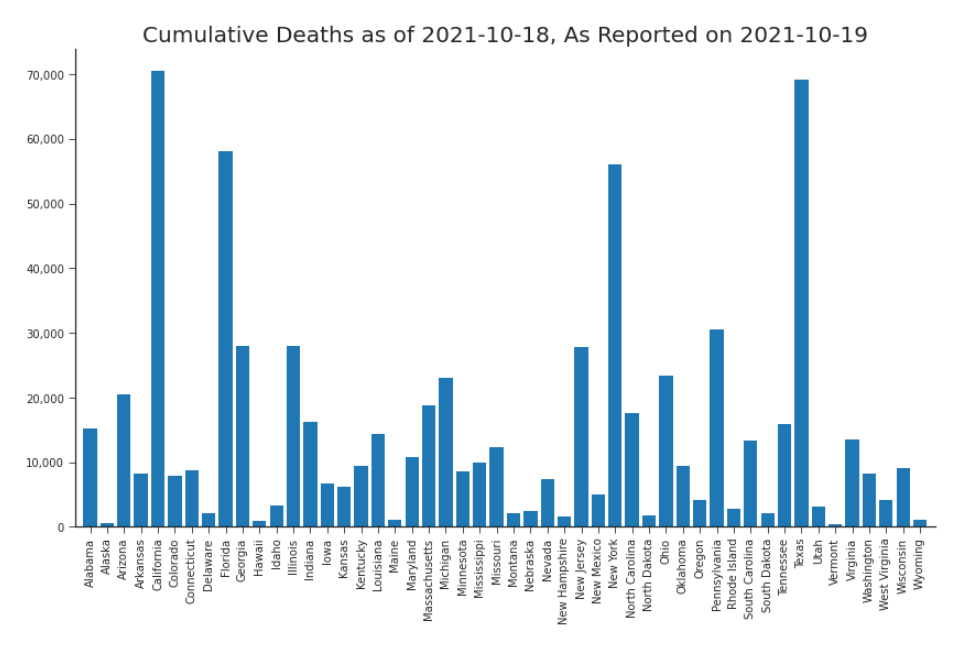
Figure 6.1. Cumulative Deaths in California as of October 18th, 2021, as Reported in October 19th, 2021 Release We could trust this data and act on it as-is. Or, we could assess its quality and use it in light of that knowledge. Suppose it’s October 20th, 2021. You are tasked with distributing COVID-19 relief funds across the states. You pull down data from JHU CSSE repository and look for the count of cumulative deaths.1 It’s the morning, so most of the data in these files was updated the day before, October 19th. Although some

For details on this data and how we curated our datasets, please see Appendix C.2.

of the states have values for October 19th, you don’t really trust those numbers because they were reported before the day had actually ended. Instead you look at the cumulative deaths for the 18th. So, on the 20th (i + 2) you’re looking at data reported on the 19th (i + 1) about the 18th (i) i+1 Xii+1 = {xi,m m ∈ M}

where M is the set of fifty states. When you’re interested in a particular state, such as California in the Prologue, you can drop the m, xii+1 . You could start distributing funds according to these numbers (Figure 6.1), but you hesitate. You’ve seen some articles questioning the US’s COVID-19 data. Before you base your decisions off this data, you’d like to know whether or not you should. You’ve done your homework (Chapter 4) and have decided that the dimensions of data quality most relevant to your task are accuracy, completeness, consistency, timeliness, validity, and believability. First, you’ll have to define what those dimensions mean to you (Figure 6.1), given that the definitions are not standardized in the literature. Next, you’ll have to define measurement for those dimensions. You were able to build off the literature for the definitions of those dimensions, but there is little guidance for measurement. There are some qualitative examples, but you don’t have time to do a qualitative assessment of the data for each of the fifty states. You have to distribute today’s funds today.2 You definitely need a quantitative measurement. You’ll have to define your own metrics.

Using terminology from Chapter 4, you might say the volatility of the data is 2 days. But that ignores the somewhat common use of older data to nowcast in place of missing data. It also glosses over the likely fill-forward data we’ve seen in the Prologue.

Definitions for Data Quality Dimensions Accuracy The degree to which the values reported sufficiently reflect the real world values Completeness The degree to which values are reported for the data elements that are required Consistency The degree to which the target definition, method of measurement, and production process remains consistent across all subsets of the dataset Timeliness The degree to which data is fit for use in the required time Validity The degree to which the dataset conforms to its intrinsic constraints Believability The degree to which data adheres to expectations, given its production process and subject matter Table 6.1: Proposed Definitions for Data Quality Dimensions These definitions are inspired by the discussion in Chapter 4, with conflicts resolved and clarity added at our discretion. You’re looking to measure the quality Q the data set Xii+1 for our finite resource allocation use case u, Q(Xii+1 , u) = (D, d)

where D is a matrix containing dimensions calculated for each of the 50 states and d is a vector of dimensions measuring the dataset as a whole. After the quality is assessed, you’ll need to summarize the quality concisely enough to inform actions. In practice, this would be done by a scoring function A(D, d) = q

where q is a vector of scores for each state. The scoring function is not a focus of this work but A ought to be considered critically in terms of the team’s risk tolerance and updated over time as it changes. In this case, the team’s tolerance for misallocation of funds should inform the scoring function. In order to inform the use, we need a score. In order to create the score, we

need to evaluate the quality. In order to evaluate the quality, we need to deal with a problem we’ve discussed but have yet to tackle: the very tricky issue of reference or truth values for accuracy. In order to do that, we’ll need the help of previous releases.

Creating Releases

The fine team at JHU CSSE continuously published up-to-date data for over three years. This created many more versions of data than there were days. In order to replicate how we’re using data in this use case, we’ve gathered the last version of data available at the end of each day.3 Once we gathered that data, we organized it into the upper triangular release matrices we’ve grown accustomed to in previous chapters. For state m ∈ M, we have Xmi+1 = {xkj,m , j = 0, …, i,

where j is the observation date, k is the release date, and the matrix is organized by observation × release.

Defining Truth

In economics, it’s common to use the most recent available data as the reference value or source of truth (Jacobs and Norden, 2011). Let’s follow suit. We can measure accuracy of a release i+1 relative to T , the last release we have available. We’ll call this T -accuracy. For now, let’s calculate accuracy as percent error of

See Appendix C.2 for details.

the value it reports for i relative to the true value (the value reported in release a(i + 1) =

xii+1 − xiT xiT

where T corresponds to the last release in our dataset, June 11th, 2022.4 Release i + 1 is perfectly accurate when a(i + 1) = 0. We can plot a by the release (Figure 6.2). A suspicious trend readily appears: newer values are more accurate.

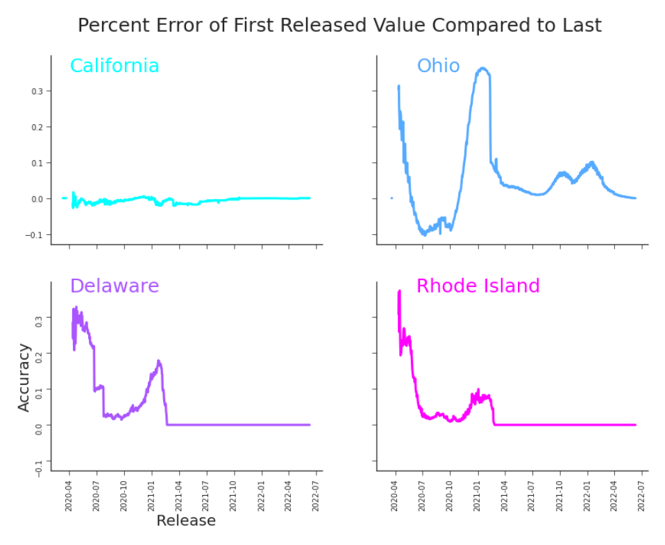
Figure 6.2. Accuracy Relative to a Popular Choice of Truth Value More recent data is more accurate. Is that a function of the data itself, or the choices we made when measuring accuracy? (Calculated according to Equation 6.1.1.) Is this a true feature of the data? Or is it simply a function of our measurement?

When examining cumulative deaths we were, unfortunately, not burdened for long with a zero denominator.

Older data has had more time to be revised. Let’s revisit a plot from Chapter 3. We’ve reproduced a between release heat map in Figure 6.3. It color codes our upper triangular matrix of releases, highlighting revisions between any release (column) and the previous release. We can follow a single observation horizontally from the diagonal to the right hand side. An earlier observation (row) has had more opportunities to be restated. Indeed, an older observation has, in general, more major restatements crossing its row than a more recent observation. Older observations have, by definition, had more opportunities to be revised. Let’s examine this another way. By rewriting the the numerator in equation xii+1 − xiT = −

(xij+1 − xij )

we see that it’s equal to the −1 times the sum of the adjustments between subsequent releases. If all data were adjusted in the same fashion, newer data would always appear more correct according to accuracy as measured by equation 6.1.1. More pointedly, according to equation 6.1.1 we would never need to estimate accuracy in practice. If release T is the latest release, then T = i + 1. We can directly calculate xTT −1 − xTT −1 xii+1 − xiT = =0 a(i + 1) = xiT xTT −1

which is the accuracy of the most recent release, and therefore the release in question. Measuring accuracy with respect to release T punishes older releases unfairly and is uselessly lenient with with recent releases. Every current release is perfectly accurate–until it’s no longer the current release. Under this measurement, accuracy of a release can constantly change.

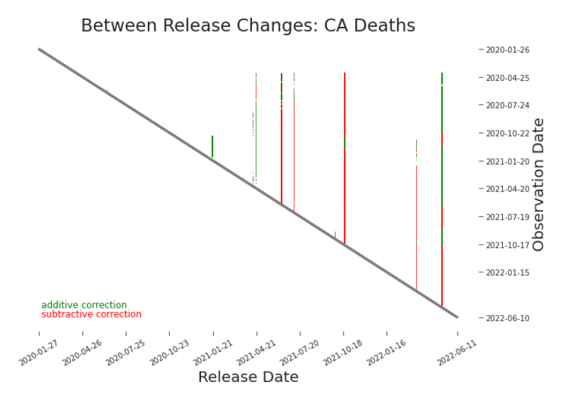
Figure 6.3. Reproduction of Between Release Heat Map Each colored cell indicates a revision. We can trace the revision history of a release by moving horizontally from the diagonal to the right hand side. The older the observation date, the more opportunities it’s had to be revised. Instead, let’s measure the accuracy of a release relative to the accepted truth at some distance κ into the future. We’ll call this κ-accuracy. Then, our calculations measure xii+1 relative to xii+κ . We’ll adjust equation 6.1.1 to accommodate these κ-accuracy truth values αi+1 i (κ) =

xii+1 − xii+1+κ xii+1+κ

where κ ∈ {1, … , T − (i + 1)}. We explore this option in Figure 6.4, with κ = 30, 90, 150, 365. The plots indicate a more ”even handed” nature to our measurement. In the T accuracy plot, reproduced in the last row of the same figure, the apparent inaccuracies of earlier releases distract from those of 2021 but they dominate all the κ-accuracy plots. A shortcoming of κ-accuracy is that we cannot directly measure the accuracy of current releases. Unlike with T -accuracy, with κ-accuracy it’s both useful and

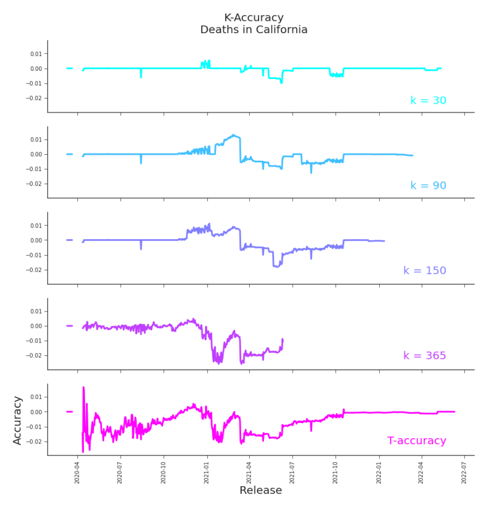
Figure 6.4. Comparison of Accuracy Using Different Truth Values In general, the smaller the κ, the better the apparent accuracy. This follows intuition, given that a smaller κ provides fewer opportunities for revision. The larger the κ, the larger the time between the last directly measurable release and the current release. By definition, we can only measure a release that is from a date at least κ-1 days prior to the current release.

feasible to estimate the accuracy of the current release. To estimate αi+1 i (κ) we rely on the previous releases

Now that we’ve found a way to estimate accuracy (Figure 6.5), we should consider how exactly we’d like to measure it and the other metrics of data quality.

Accuracy

We’ve already proposed one metric for κ-accuracy, equation 6.1.1. But, there are many potential options worth considering. For example, we consider the indicator function:

1{xii+1 = xii+1+κ } . The metric has a convenient range, [0, 1], and is immediately interpretable. However, it’s not very actionable. Although perfectly accurate data would be nice, it’s not needed for this use case. We need sufficiently accurate data, such that we can distribute funds reasonably well. We need to know how imperfect our data is, not whether or not it is perfect. (We already know that it’s not.) Alternatively, we could consider absolute error |xii+1 − xii+1+κ | to assess accuracy. However, we’re looking at death counts of very different scales (see Figure 6.1). We may assume that errors are a function of total deaths, i.e. we expect larger absolute errors for larger absolute numbers of deaths. If that’s the case, this metric unfairly penalizes states with large death counts. Absolute deaths would be more relevant if, say, the error mechanism was due to an engineering error. For example, if rows of data were occasionally dropped at the last step

of the aggregation. If the those rows were dropped independent of the size of the data, then using the absolute error might be more appropriate. But we have no reason to expect such a mechanism to be driving these errors. From Chapter 2, we expect errors to occur upstream in the production process, somewhere in the tangled web of hand-offs between the overworked and under-resourced American healthcare and public health systems. Alternatively, we could use the squared error, (xii+1 − xii+1+κ )2 . This error harshly penalizes large absolute errors but at the cost of losing direct interpretation. Unfortunately, it is even more susceptible to changes in size than the total error calculation. This metric has the additional downside of losing directionality. For our use case, it would be very helpful to know if the data is over-reporting or under-reporting deaths. In the former case, we’d be wary of sending funds to a state that we may later need to claw back. In the latter, we may reserve funds as we anticipate needing to send more. A successful metric will retain directionality but will be robust against the scale of the κ-accuracy truth value. The previously proposed percent error, Equation 6.1.4, fits the bill, αi+1 i (κ) =

xii+1 − xii+1+κ xii+1+κ

Now that we know what we want to measure, we need to estimate it.

Estimating Accuracy

On day i + 2, the most recent release we have is i + 1. We can only measure the accuracy of releases j at least κ days prior: {0, … , i + 1 − κ}. Therefore, we can

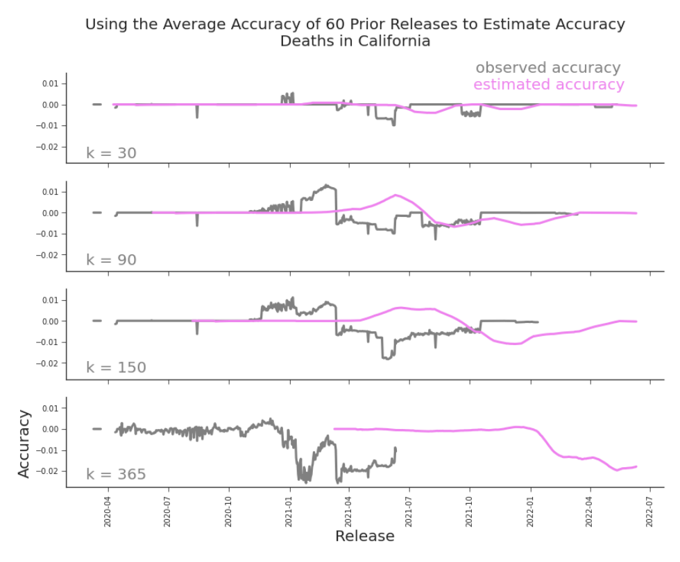
Figure 6.5. Estimating Accuracy Localized accuracy issues impact estimates κreleases into the future. only estimate the accuracy of release i + 1 with the set of i + 1 − κ releases. We have the data, but unfortunately we do not have a distribution for the errors. In particular, we’ve seen that the errors are not well-behaved (Figure 6.4). We will try a simple mean of the most recent n available accuracies to estimate αi+1 i (κ) α̂i+1 i (κ) =

i−κ 1 X j+1 α (κ) . n j=i−κ−n j

In Figure 6.5, we can see that deviations in observed accuracy only impact the estimated accuracy for releases at least κ-days into the future. From Figure 6.5, it’s clear that this estimate does not perform particularly well. Large sections of accuracy failures hurt this estimate’s performance. Those blocks are caused by news in the form of major restatements. With news, we don’t expect to nowcast the values well and we don’t expect to estimate the accuracy particularly well either.

Suppose that on day 90, California changes its data definition. They move from reporting the sum of confirmed and probable deaths to only reporting confirmed deaths. They apply this change retroactively, restating all previously reported values. Using κ = 30, the accuracies of releases 60 − 89 will look artificially bad. Those releases report the sum of confirmed and probable deaths. But the accuracy measurement compares them to releases 90 − 119, which report only the confirmed deaths. So, using the observed accuracy of releases 60 through 89 to estimate the accuracy of any release 90 or after should introduce error. Fortunately, we can identify whether release 90 is a major restatement as soon as it is released. We introduced major restatements in Section 3.2.1. There we observed major restatements that rewrote nearly all of history. We saw them appear as solid vertical bars in the between release plots (Figure 6.3). Not surprisingly, this sort of near-complete rewriting of history impacts κ-accuracy. A major restatement is a release that revises history to the point that it impacts the use of the data (as determined by application). In this case, let’s define that to be at least β percent of the previous release’s values. That is, if a release rewrites enough history, we may be concerned that it has introduced a change in definition or production such that its values are no longer comparable to other states. Release i + 1 is a major restatement for a given state if i−1

equals 1. In Figure 6.6 we’ve set β = 0.20. A major restatement that occurs in release i + 1 cannot impact the accuracy of release i + 1 or subsequent releases. However, accuracy estimates for releases i + 1 forward could rely on the impacted releases (releases i + 1 − κ to i). Unless the major restatements themselves are predictable, we do not expect to accuracy estimates to capture the impact of major restatements. In general, we expect major restatements to be news. Therefore, it is critical to consider major restatements when interpreting κ-accuracy.

Completeness

Suppose that on day 91 we open up release 90 to find that California does not have a value reported for day 89. Does this prevent us from sending funds to the other 49 states? Hopefully not. Perfect completeness is not necessary to act, but more complete data is certainly better. A popular measure of completeness of a datum is binary. For us, this would mean measuring the completeness of a release i + 1 for state m with i+1 1{xi,m is not Null}.

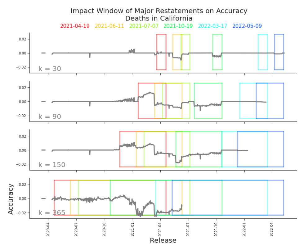
Figure 6.6. Impact Window of Major Restatements on Accuracy, Deaths in CA Each box is created by placing a vertical bar at a major restatement and capturing the κ-releases prior to (to the left of) it. The box encases the releases whose accuracies are impacted by that major restatement. As κ increases, the rectangles widen to the left. Looking at the major restatement from 2021-10-19, there are clear and contained impacts to the 30-day and 90-day accuracies. Either a value is reported or not. We need to consider the data as a whole as well. We could use the product of this binary metrics to assess the release i + 1,

i+1 1{xi,m is not Null}.

Conveniently it shares a domain with the binary metric. But it requires perfect completeness of a dataset, which is not required for the task at hand. This metric would prevent us from using very usable datasets.

Instead, we can measure the percent completeness of release i + 1 across M using i+1 Σm∈M 1{xi,m is not Null}

which communicates the nuance of imperfect-but-usable. Notably, we are not evaluating the presence of historic values, xi+1 j for j ≤ i. Our concern is xii+1 . But, if that value is missing, we may be able to lean on those earlier values xi+1 j , j < i.

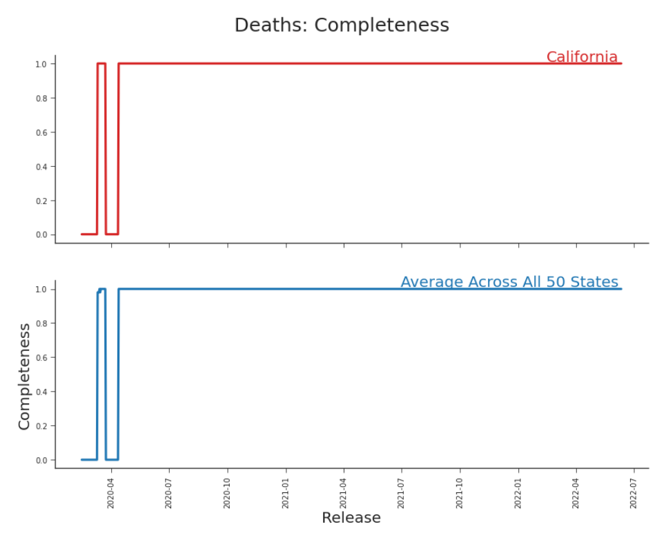
Figure 6.7. Completeness, Deaths in CA Compared to the Average Across States We have exceptionally complete data, save for a few days early in the pandemic when reporting was being sorted out. Given what we observed in the Prologue and learned in Chapter 2, this is suspiciously perfect. In Chapter 7 we’ll discuss fill-forward behavior and why apparent completeness is sometimes a trick of the data.

Completeness and Timeliness: Lateness

Suppose again that it is day 91. Release 90 has no value reported for cumulative deaths as of day 89 in California. We could withhold funds completely. We could just withhold funds from California. Or, knowing that these are cumulative counts, we could rely on the count reported for day 88. After all, cumulative deaths are non-decreasing. The count for day 89 should have a lower bound of day 88’s tally. If there’s no value for day 88, then we would look to day 87 and so on. Of course, our faith in this very primitive nowcasting is low. It gets lower the further back we have to reach for a value. We’ll use the term lateness to refer to this combination of (in)completeness and timeliness. We can measure the lateness of a particular state within a release using (1 −

where 1 indicates xii+1 is reported and 0 indicates the release is empty. This metric has the nice feature of penalizing lateness less as the pandemic goes on. This coordinates well with the cumulative counts which, all things being equal, are expected to increase less as a percentage of the total later in the pandemic. We could measure lateness by simply counting the number of days late our data is i − j where j = max( j) s.t. ∃xi+1 j . This has the nice feature of being directly interpretable. But in order to contextualize that number, the reader must have a sense of the total number of days that reporting has been going on. Additionally, it penalizes lateness equally across the duration of the pandemic.

Figure 6.8. Lateness, Deaths in CA Mimicking Figure 6.7, California is nearly perfect in it completeness. The difference between lateness and completeness appears only in the pizza-slice cut out from the upper left hand block. In that cutout, we see how far back in history we have to reach to get the most recent reported value.

Timeliness and Accuracy

Suppose on day 91 you have a perfectly complete release 90. But, the value reported for day 89 is wrong. Very wrong. It would make the dataset worse than useless, because the data looks perfect. It would give the user the confidence of having great data. But using data that wrong with that much confidence would be worse than using no data at all. It’s not enough to have data or to have that data in time to use it. The data also needs to be reasonably accurate. As we’ve discussed in Section 4.4.3, there’s often a trade-off between getting data quickly and getting accurate data. As a result, we often have data that arrives on time but is not very accurate. Suppose, as in Section 6.5, we are missing the xii+1 value and we need to use a value for an earlier observation date. We’d prefer that earlier value to be reasonably accurate.

We can measure how long it will take until the value reported for an observation i is sufficiently accurate, or ϵ-accurate. We calculate ti = min(k) s.t. |αii+ j (κ)| < ϵ ∀ j k ≤ j ≤ κ.

Because this relies on accuracy, we cannot measure this at time i + 1. Instead we estimate it using previous releases tˆi =

In a similar fashion to our accuracy estimations, this calculation is impacted by the presence of major restatements. It is critical that we consider these estimates in light of major restatements as well.

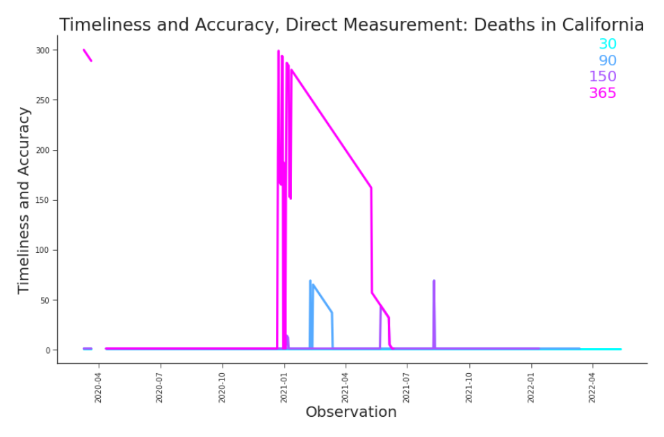
Figure 6.9. Timeliness and Accuracy, Deaths in CA The diagonal lines capture the impact of major restatements on accuracy. Their shape echoes those diagonal lines that indicate major restatements in lag plots. See Figure 6.10 below.

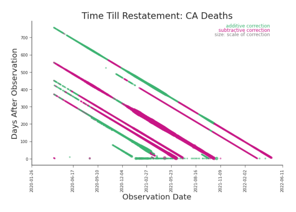
Figure 6.10. Reproduction of Lag Plot: Deaths in CA The major restatements reveal themselves as diagonal lines. (Reproduced for convenience from Figure 3.14).

Consistency

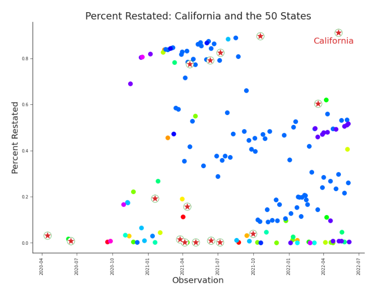
Figure 6.11. Percent Restated, California Amid the States By plotting the percent restated in each release, we see that states are indeed actively revising earlier data. For purposes of visual discovery, we have removed points associated with percent restated = 0, which (expectedly) dominate the releases.

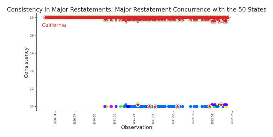
Figure 6.12. Consistency in Major Restatements Most releases do not constitute a major restatement for any given state. Thus, they are highly concurrent. When a state does have a major restatement, it’s notable in its divergence from the pack and even more notable when it has company. Suppose on day 91, release 90 contains two types of values. Half the states reported confirmed deaths, half the states reported the sum of confirmed and probable deaths, and all the values recorded are in the same column, simply labelled ”deaths.” It would make distributing funding equitably error prone, although wouldn’t know it. Ideally, all states would be reporting the same underlying measurement (e.g. confirmed deaths). Our hope for consistency is that xi,i+1j represents truth in the same way that i+1 xi,m does. One way we can assess consistency of a release i + 1 is to assume that

prior to this release, all states were reporting the same underlying truth.6 Then, if a major restatement occurs, it hopefully happens across all states concurrently. We can measure the concurrence of major restatements across regions of interest

This assumption, of course, is prone to fail.

M = the set of regions m, with Ri+1 = 2 ×

1 X i+1 r − .5 |M| m∈M ·,m

which is close to 0 when about half the regions have major restatements and close to 1 when most of the regions align. We can assess the alignment of a state m′ with the larger set of regions i+1 1 − r·,m ′ −

ri+1 |M| − 1 m∈M,′ ·,m

which is near 0 when m′ differs from all other states and 1 when all states align.

Validity and Believability

Recall from Section 0.1, that on June 10th, 2021, three-hundred and thirty-nine Californians rose from the dead. What otherwise might have inspired some choruses shook our faith in the data. Deaths are, in general, quite final after all. A simple but very helpful rule for cumulative deaths is: cumulative deaths should not decrease over time. When they do decrease, as on June 10th, we start questioning our data. Without having to plot all fifty states each day, we can simply monitor this measure of believability and validity. For a release i + 1 and state m, we measure i+1 1{xii+1 ≥ xi−1 }

which is 1 if the constraint is satisfied and 0 if it is violated. Of course, there are other measures of validity and believability that we could consider. For example, cumulative deaths should not exceed the population of a state. Or, cumulative deaths should not exceed cumulative cases.

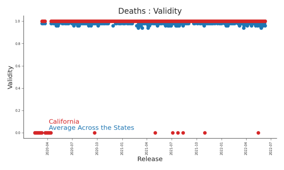
Figure 6.13. Validity, Deaths in CA Decreasing values in a cumulative count calls into question how much we really believe our data. As we’ve seen, there are few days in California that the are hard to believe. There are any number of possible signals for belivability and validity. We chose this one because it can be calculated within the dataset of releases and without any external data for comparison, which removes the reliance on data quality of external datasets. We could also consider a metric indicating that no revisions have been made. Given the data production process, we expect that many of the first released values will need to be revised. If a state is either unwilling or unable to correct previously reported values, it calls into question their entire data production process. It may be worthwhile to hold in suspicion data from any state that neglects to correct previous reporting.

Dimensions Accuracy Completeness Completeness: Average Across States Completeness and Timeliness Timeliness and Accuracy Consistency: Major Restatement Consistency: Concurrence Consistency: Across States Validity

Target Range i+1 (− inf, inf) xii+1 {0, 1} i+1 {xi,m } (0, 1) i+1 (0, 1) xi+1 1, … , κ i+1 {xi,m } {0, 1} i+1 i+1 xim ∈ {xi,m } (0, 1) i+1 {xi,m } (0, 1) i+1 {0, 1}

Table 6.2. Proposed Dimensions for DQ Assessment for the Allocation of Finite Resources Across the Fifty States. 2021-10-19 Estimated Accuracy Estimated Accuracy SE Estimated Timeliness and Accuracy Estimated Timeliness and Accuracy SE Completeness Completeness: Average Across States Completeness and Timeliness Consistency: Restated Percent Consistency: Major Restatement Consistency: Major Restatements Consistency: Major Restatement Concurence Consistency: Across States Concurence Validity Validity: Average Across States

Dimensions	Target	Range	Goal	Eq.
Accuracy	x_i^(i+1)	(−inf, inf)	0	6.1.4
Completeness	x_i^(i+1)	{0, 1}	1	6.4.1
Completeness: Average Across States	{x_(i,m)^(i+1)}	(0, 1)	1	6.4.2
Completeness and Timeliness	x^(i+1)	(0, 1)	1	6.5.1
Timeliness and Accuracy	x^(i+1)	1, …, κ	1	6.6.1
Consistency: Major Restatement	{x_(i,m)^(i+1)}	{0, 1}	1	6.3.2
Consistency: Concurrence	x_(i,m)^(i+1) ∈ {x_(i,m)^(i+1)}	(0, 1)	1	6.7.1
Consistency: Across States	{x_(i,m)^(i+1)}	(0, 1)	1	6.7.2
Validity	x^(i+1)	{0, 1}	1	6.8.1

Table 6.3. Real-Time DQ Assessment of Deaths in CA, Release 2021-10-19 with κ = 90 This release was identified as a major restatement, presenting a near complete revision of history.

	2021-10-19
Estimated Accuracy	0.000
Estimated Accuracy SE	0.000
Estimated Timeliness and Accuracy	4.176
Estimated Timeliness and Accuracy SE	0.571
Completeness	1.000
Completeness: Average Across States	1.000
Completeness and Timeliness	1.000
Consistency: Restated Percent	0.897
Consistency: Major Restatement	1.000
Consistency: Major Restatements	4.000
Consistency: Major Restatement Concurence	0.000
Consistency: Across States Concurence	0.960
Validity	1.000
Validity: Average Across States	1.000

Evaluating a Day’s Data

Let’s assume it’s October 20th, 2021 and we are working with the committee to allocate funds to aid in the response to COVID-19 deaths. We happen to represent California, so we are going to pay particular attention to the Golden State. We are evaluating the fitness of the data to help guide these decisions. We are looking at the cumulative deaths as of October 18th as reported in the October 19th release. We need to send funds by the end of the day, so we better get rolling. We evaluate this release using the metrics proposed throughout this Chapter. Table 6.9 contains the observed and estimated values. In addition, we’ve included the standard error of the estimates. We notice that our two estimated metrics seem to contradict each other. The first, estimated accuracy, indicates that we should trust the value. The second, estimated timeliness and accuracy, indicates that we shouldn’t expect this value to be correct for a few more days. On its surface this seems contradictory. Then, we see that this is a major restatement. In fact, this is the fourth major restatement in California already. And, with κ = 90, a major restatement can impact the accuracy of values reported 90 days prior. That means that the timeliness and accuracy metric is likely being inflated by those major restatements. The major restatements are not large in their corrections of historic values, else accuracy would have been worse. It looks like California’s value is likely pretty accurate. Fortunately we have values reported for all 50 states. California is the only state with a major restatement in this release. This restatement rewrote almost 90% of California’s history. It raises some questions about the comparability of this data to the other states. In order to understand why California revised so much of its data while most other states did not, we ought to reach out to the data producers and subject matter experts for more context.

We first look to the data curators at JHU CSSE. In their GitHub repository, we find a note in the README.md file under Data Modification Records for October 19th, 2021: ”Adjust California’s death data based on historic data provided by CDPH.” We’re confident this revision was purposeful on the part of the data curators. Now we’ve got to reach out to the California Department of Public Health (CDPH) to understand why they changed the data. Technological infrastructure can be implemented so that these metrics are calculated effectively instantaneously as soon as the data is published or, in this case, just after midnight. We’ve now defined our data quality assessment Q(Xii+1 , u) = (D, d)

The practitioner is left to define a score function A(D, d) = q tailored to the specific risk tolerance and decision-making method. A practical example of a score function would be a three-level alert system built on explainable business rules and statistically-backed sensors. For the purpose of demonstration, we’ve built a simple and effective one, the details of which can be found in the Appendix. With a good score function, we don’t need to review the DQ metrics for each of the 50 states every single day; we only need to respond to any alerts that are triggered (Figure 6.14). It’s no surprise that California has raised an alert: it underwent a major restatement and has a large timeliness and accuracy estimate. After reaching out to CDPH, we’ll want to follow up on the quality metrics for the other states that triggered alerts: Delaware, Indiana, Ohio, Rhode Island, Texas, and Washington state (see Appendix B.1). Then, we can distribute funds with confidence where we can and cautiously where we must.

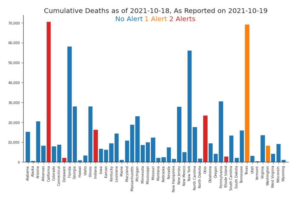
Figure 6.14. A DQ-Informed View of Cumulative Deaths in California as of October 18th, 2021, as Reported in October 19th, 2021 Release With our metrics defined and a scoring function in place, we can color code our initial plot (Figure 6.1) according to alerts raised, which signal DQ concerns. Now we are able to use our data in light of its quality.

---

Notes

1. When not otherwise stated, we can let n = i−κ and use the entire available history to estimate accuracy: α̂i+1 i (κ) = f (α0 (κ), … , αi−κ (κ)).